Shifts In Aggregate Spending Function
Shifts In Aggregate Spending Function Assignment Help | Shifts In Aggregate Spending Function Homework Help
Shifts In Aggregate Spending Function
Equilibrium level of national income is attained where the aggregate expenditure equals GDP. While 450 line or GDP curve remains unmoved, the AE curve may shift upwards or downwards due to changes in its constituents. A shift in AE curve will cause an increase or decrease in the GDP.
For any AE line there is a unique equilibrium level of GDP. In case, the AE line shifts, it will disturb the equilibrium level of GDP. A change in GDP causes a movement along the AE curve. An increased desire to spend at each level f GDP causes a shift in the aggregate spending line. AE line will shift, when there is shift in the consumption function or desired investment spending.
For any AE line there is a unique equilibrium level of GDP. In case, the AE line shifts, it will disturb the equilibrium level of GDP. A change in GDP causes a movement along the AE curve. An increased desire to spend at each level f GDP causes a shift in the aggregate spending line. AE line will shift, when there is shift in the consumption function or desired investment spending.
Upward Shifts in the Aggregate Spending
Upward shifts in the aggregate spending take place when: (i) the individual household permanently increase their consumption spending at each level of disposable income and (ii) When the firms spend more on investment. e.g., inventory accumulation, more investment on fixed capital, etc.
An upward shift in the aggregate spending function means that the desired spending at each level of national income raises to and stays at a higher amount.
Two types of shifts can take place in the AE curve; these are:
First, the same addition to spending occurs at all level of income. In this case, the AE curve shifts parallel to itself as shown.
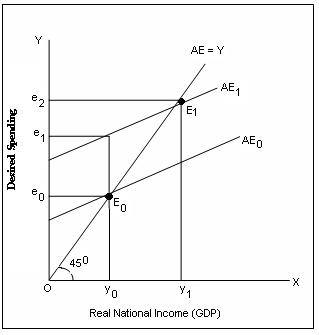
In point E0 is the equilibrium level of national income where the initial aggregate spending curve AE0 intersects 450 line.
A parallel upward shifts in aggregate spending is shown by AE1 which is parallel to AE0.
The parallel upward shift in the AE line from AE0 to AE1 means that desired spending has increased by an equal amount at each level of national income. For example, at national income Y0, the desired spending increases from e0 to e1, therefore, exceeds aggregate output (GDP). E equilibrium is reached at E1, where national income (output) raises to Y1 and spending is e2. The increase in desired spending from e1 to e2 is shown by moment along AE1, It is an indicued response to the increase in GDP from Y0 to Y1
Second. if there is a change in the propensity to spend out of national income. In this case, the slope of the AE line changes (i.e., marginal propensity to spend changes). Such a change occurs when the households decide to spend more of every rupee of (Z) is shown.
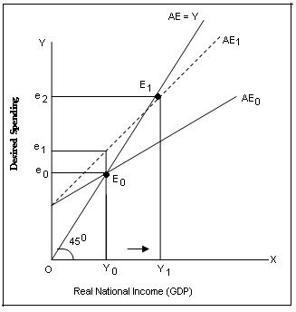
In equilibrium level of national income is attained at E0, where the initial AE0 curve intersects 450 line. Non-parallel shift in AE is shown by the new AE1 curve. It shows that the marginal propensity to spend at each level of national income has increased, therefore, the slope of AE1 has changed. The new equilibrium level of national income is reached at E1, where the new AE1 curve intersects 450 line. The new level of desired spending rises to e2 and national income to Y1.
An upward shift in the aggregate spending function means that the desired spending at each level of national income raises to and stays at a higher amount.
Two types of shifts can take place in the AE curve; these are:
First, the same addition to spending occurs at all level of income. In this case, the AE curve shifts parallel to itself as shown.
In point E0 is the equilibrium level of national income where the initial aggregate spending curve AE0 intersects 450 line.
A parallel upward shifts in aggregate spending is shown by AE1 which is parallel to AE0.
The parallel upward shift in the AE line from AE0 to AE1 means that desired spending has increased by an equal amount at each level of national income. For example, at national income Y0, the desired spending increases from e0 to e1, therefore, exceeds aggregate output (GDP). E equilibrium is reached at E1, where national income (output) raises to Y1 and spending is e2. The increase in desired spending from e1 to e2 is shown by moment along AE1, It is an indicued response to the increase in GDP from Y0 to Y1
Second. if there is a change in the propensity to spend out of national income. In this case, the slope of the AE line changes (i.e., marginal propensity to spend changes). Such a change occurs when the households decide to spend more of every rupee of (Z) is shown.
In equilibrium level of national income is attained at E0, where the initial AE0 curve intersects 450 line. Non-parallel shift in AE is shown by the new AE1 curve. It shows that the marginal propensity to spend at each level of national income has increased, therefore, the slope of AE1 has changed. The new equilibrium level of national income is reached at E1, where the new AE1 curve intersects 450 line. The new level of desired spending rises to e2 and national income to Y1.
Downward Shifts in Aggregate Spending
Downward shift in aggregate spending occurs when there is decrease in consumption spending or in investment spending. Because of a fall in the aggregate spending the AE curve will shift downward shift in the AE:
First. a constant reduction and desired spending at all levels of national income. In this case, AE curve shifts downwards parallel to itself.
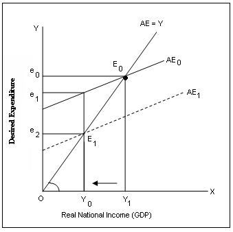
In equilibrium level of national income is attained at E0, where the initial AE0 curve intersects 450 line. After a constant reduction in aggregate spending, the AE curve shifts downwards to AE1. A fall in aggregate spending causes decrease in the level of output and income. The new equilibrium level of national income is attained at a lower level Y1, and lower level of aggregate spending e2.
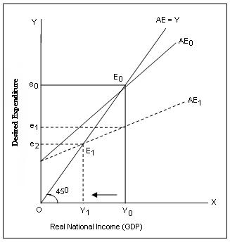
Second. a fall in marginal propensity to spend (Z), out of national income. It will reduce the slope of the AE line. This kind of change in desired spending occurs when the households decide to spend less of every rupee of disposable income. The effect of a downward shift in aggregate spending is shown.
In the equilibrium level of national income is shown by E0, where to initial AE0 curve intersects 450 line. After a fall in aggregate spending with marginal propensity to spend diminishing, the slope of the AE curve changes so that non-parallels AE1 curve shifts downwards. The new equilibrium level of national incomes reached at E1 where the desired spending falls to e2 and the level of national income also falls to Y1.
For more help in Shifts In Aggregate Spending Function click the button below to submit your homework assignment
First. a constant reduction and desired spending at all levels of national income. In this case, AE curve shifts downwards parallel to itself.
In equilibrium level of national income is attained at E0, where the initial AE0 curve intersects 450 line. After a constant reduction in aggregate spending, the AE curve shifts downwards to AE1. A fall in aggregate spending causes decrease in the level of output and income. The new equilibrium level of national income is attained at a lower level Y1, and lower level of aggregate spending e2.
Second. a fall in marginal propensity to spend (Z), out of national income. It will reduce the slope of the AE line. This kind of change in desired spending occurs when the households decide to spend less of every rupee of disposable income. The effect of a downward shift in aggregate spending is shown.
In the equilibrium level of national income is shown by E0, where to initial AE0 curve intersects 450 line. After a fall in aggregate spending with marginal propensity to spend diminishing, the slope of the AE curve changes so that non-parallels AE1 curve shifts downwards. The new equilibrium level of national incomes reached at E1 where the desired spending falls to e2 and the level of national income also falls to Y1.
For more help in Shifts In Aggregate Spending Function click the button below to submit your homework assignment