Price Discrimination

There are more possibilities for a monopolist to take advantage of his/her situation: She can charge different prices from different customers. This is called price discrimination, and we distinguish between price discrimination of the first, second, and third degrees.

First Degree Price Discrimination

Remember that the demand curve corresponds to the consumers’ valuation of different quantities of the good. Suppose, for example, that we have four presumptive consumers who want to buy a maximum of one unit of the good. The first is willing to pay 4 for one unit of the good, the others 3, 2, and 1, respectively. We then get a demand curve as D: If the price is 4, we sell one unit to the first customer, if it is 3 we sell one unit to each of the first two, and so on. We have indicated the reservation prices of each customer with a star and then joint them with a straight line.

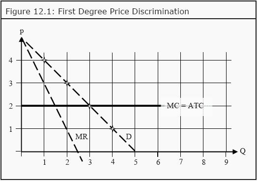
Furthermore, assume that the monopolist has a constant marginal cost, MC = 2, and no fixed cost. Then AVC = ATC = MC. In a perfectly competitive market, the equilibrium price would have been p* = 2 and the quantity sold would have been Q* = 3. The firm’s revenue would have been 3*2 = 6 (Q*p), and its cost 3*2 = 6 (Q*ATC). Its profit would therefore have been zero. The consumer surplus (CS) would have been the sum of each customer’s surplus, i.e. the difference between his or her valuation and how much he or she pays. For the first customer, the surplus is 4 - 2 = 2, for the second 3 - 2 = 1, and for the third 2 - 2 = 0. Therefore, we get a total consumer surplus of CS = 3. In a monopoly market of the type, the firm would have found the quantity at which MC = MR, i.e. Q = 1.5. If it can only sell whole units, it would have chosen to produce only one unit that it would have sold at a price of 4. The profit (= PS) would then be 1*(4 - 2) = 2, which is higher than in the perfectly competitive case. CS would be 4 - 4 = 0. Suppose now instead that the monopolist knows the valuation of each consumer, and that the consumers cannot sell the goods to someone else if they have bought it. The monopolist can then use price discrimination of the first degree (also called perfect price discrimination): She charges a price from each customer that is equal to the maximum amount that customer is willing to pay.
The first customer has to pay 4, the second 3, and the third 2. Since the monopolist has a marginal cost of production equal to 2, her surplus will be PS = (4 - 2) + (3 - 2) + (2 - 2) = 3. CS will be 0. Compared to a perfectly competitive market, the monopolist has won over all the CS. Note that in this case, with first-degree price discrimination, the social surplus is as just large as in the case of perfect competition. The surplus has just been reallocated from the consumers to the producers. This means that this situation is actually efficient. It is another question whether it is fair.

Second Degree Price Discrimination

If the monopolist does not know the different valuations of different customers, she can instead use second-degree price discrimination. This amounts to offering different package solutions at different prices, and then the customers get to choose which package they prefer. By choosing the composition of the packages in a clever way, she can get the customers to sort themselves into different groups. The goal of making them perform this type of self-sorting is to get the ones with high valuation to pay a high price and the ones with low valuation a lower price. An example of this type of price discrimination is quantity discounts.

Third Degree Price Discrimination

The third type of price discrimination amounts to dividing the market into two or more submarkets, where the valuations in the submarkets are different. Examples are different prices for children and grownups, or discounts for students and the unemployed. For this to work, it has to be possible to identify the consumer as actually belonging to a certain group.
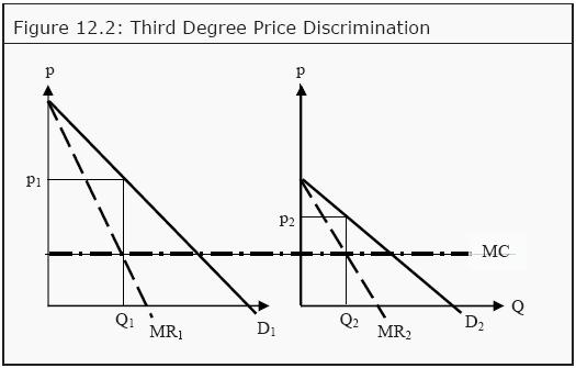
The criterion for profit maximization under third degree price discrimination is, in principle, the same as before, but we have to separate demand and marginal revenue in the two (or more) submarkets. Mathematically, this can be written as

In other words, the marginal cost of producing the total quantity has to be as large as the marginal revenue from the first submarket, and simultaneously as large as the marginal revenue from the second submarket. With constant MC and linear demand in both submarkets, this can be illustrated as in Figure 12.2. The firm chooses to produce the quantity Q₁ + Q₂, and then sell the quantity Q₁ at a price of p₁ in the first submarket and the quantity Q₂ at a price of p₂ in the second submarket.

For more help in Price Discrimination click the button below to submit your homework assignment