ALTERNATIVE GRAPHIC REPRESENTATION OF MULTIPLIER

The multiplier can also be graphically shown using the saving investment approach. In Figure 6.3, the saving (S) and the investment (I) curves intersect each other at point ‘E0’. Hence, the equilibrium level of income is OY0 . Now , suppose the investment increases by ΔI, so that the new investment curve 1 + ΔI  intersects the saving curve (S) at point ‘E1’. Thus, the new equilibrium level of income becomes OY1. The income rises from OY0 to OY1 in response to an initial increase in investment of E1 F (ΔI). It is clear from the figure that the increase in the income (ΔY) is greater than the increase in the investment (ΔI). The ratio ΔY/ΔI = K is the multiplier. In this figure, the slope of the saving curve (S) is E1 F/E0F or ΔI/ΔY.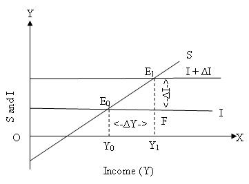

Figure 6.3: Graphic Illustration of Multiplier

But, we know that the slope of the saving curve is ΔS/ΔY or the MPS therefore,

                      ΔI     =  MPS
                      ΔY

                        ΔY    =      1
                        Δ I           MPS

Change in the Aggregate Income = Multiplier * Change in the Initial Investment. Given the change in the initial investment and the value of the multiplier, the change in the aggregate income can be found out.

For more help in ALTERNATIVE GRAPHIC REPRESENTATION OF MULTIPLIER please click the button below to submit your homework assignment.