The Individual Demand Curve

 It is possible to find the point of utility maximization if one knows a consumer’s preferences, the prices of the goods, and her budget. Let us now do that, but vary the price of good 1 and see what effect that has on, q₁, the quantity demanded.

Suppose we hold the price of good 2 (which you can think of as “all other goods”) constant. Then the effect of varying the price of good 1 will be that the budget line rotates about the intercept on the Y-axis and intersects the X-axis at different points m/p1i, where p_1i is the price one has chosen for good 1.

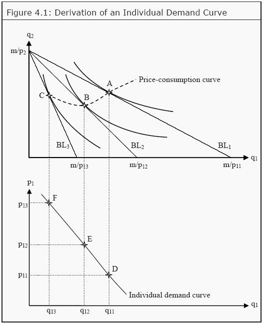
Look at the upper part of Figure 4.1. Suppose the price of good 1 is initially p₁₁. Then the budget line is BL₁. We find the indifference curve that just touches that budget line and label the point where it does so, point A. If we would raise the price of good 1 to p₁₂, the possible choices become limited to BL₂ (that intersects the X-axis in m/p₁₂) and then the consumer maximizes her utility in point B. If we continue to raise the price to p₁₃, and repeat the maximization, we get point C. If we would repeat this procedure for all possible prices, we would get a curve that is called the price-consumption curve. It shows how the optimal choice of quantity of good 1 varies with the price of that good, given that preferences, other prices and the income are held constant.

As you can see in the figure, the consumer will usually buy less of the good when the price increases. This is, however, not necessary. To see that, imagine that the indifference curve that runs through point B had been steeper. If it had been steep enough, it would touch BL₂ so far to the right that it would also be to the right of point A.

Now we want to find the demand curve for good 1. To that end, we indicate the prices we used for good 1 on the Y-axis in the lower graph of the figure, i.e. p₁₁, p₁₂, and p₁₃. Then we check which are the corresponding quantities demanded in the upper graph, at points A, B, and C, and indicate them on the X-axis in the lower diagram. (Note that both diagrams have q₁ on the X-axis.) After that, we find the points where the quantities and the corresponding prices in the lower diagram intersect, the points labeled D, E, and F. Finally, we draw a line through those points and fill in for all those numerous points for which we have not done the analysis. This curve is the individual’s demand curve for good 1.

To get more help in Individual Demand Curve click the button below to submit your homework assignment