The Transformation Curve

If we take all points along the production contract curve and calculate which combinations of goods they each correspond to, and then use that information in a new graph, we can derive the so-called transformation curve (also called the production-possibility frontier). The point from the example above, 50 fish and 100 coconuts will then be one point on the transformation curve. On the curve, we have all efficient production possibilities and underneath it, we have all other possible, but inefficient, production possibilities.

Consider point a under the transformation curve in Figure 18.4. What is the opportunity cost of producing one more unit of either good 1 or good 2? Since point a is not efficient, we do not have to give up anything to move to, for instance, point b. We just have to decrease the degree of waste in the economy. Consequently, the opportunity cost is zero! However, when we have reached point b, we cannot increase the production of good 2 more without reducing the production of good 1. If we want to move from point b to point c, we, instead, have to give up a certain quantity of good 2 to compensate for the increase in good 1. The quantity we have to give up is the opportunity cost. In other words, on the transformation curve the two goods have a price in terms of the other good, a relative price. Note that the slope of the transformation curve is defined as the marginal rate of transformation, MRT. To find MRT, we then used prices: MRT = -p₁/p₂. However, in the transformation curve there are no prices. Here, instead, we directly get the relative price of the goods. The example we used there was that one ice cream costs 10 units (of the appropriate currency) and a pizza 20 units. If we insert those prices into the formula, keeping all units, we get

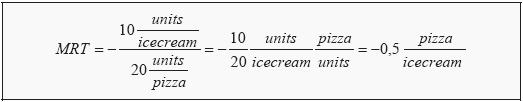
MRT is consequently the relative price for one good, expressed in units of the other good. Note that this means that the slope of the budget line is directly related to which point on the transformation curve one has chosen.

Pareto Optimal Welfare

We will now put production and consumption together in one diagram. We start from the transformation curve, and assume that society has come up with an efficient mix of goods 1 and 2, i.e. of coconuts and fish in our example. The production will then lie on a point on the transformation curve, for instance point a in Figure 18.5. The marginal rate of transformation, MRT, is the slope in point a, and we produce the quantity q₁ of good 1 and q₂ of good 2. Robinson and Friday now have to allocate the goods between themselves. We therefore add an Edgeworth box under the transformation curve, with one corner at point a and the opposite one at the origin. An efficient allocation then requires that their respective relative valuations of the goods are equal, i.e. that MRS_R = MRS_F (where the subscripts refer to Robinson and Friday, respectively). In the figure, two such allocations are indicated: point b and point c, that both lie on the contract curve. We now have efficiency in production (since the total production is on the transformation curve) and efficiency in consumption (since the allocation is on the contract curve). Is that enough for us to have general efficiency? No, it is not. It is also required that we produce what the consumers demand. There is one big difference between points b and c. In point b, the slope of the indifference curves, MRS, is the same as the slope of the transformation curve, MRT, in the point at which we have chosen to produce. That is not the case at point c. At point c, MRS is smaller in magnitude than MRT.

To see what the problem with that is, think of what MRS and MRT are. MRS is the price the consumer are willing to pay for one good in terms of the other, i.e. how many coconuts Robinson and Friday are willing to trade for one fish. Equilibrium in consumption demands that they have the same valuation. MRT, on the other hand, is the price the producers have to pay (given that the production is efficient) to produce one more unit of one good, again in terms of the other good. If the consumers are willing to pay more for one good than they have to, there are unexploited opportunities and the situation cannot constitute a general equilibrium. If we change the production such that we produce more of the good of which the consumers have a high valuation, then at least one consumer will be better off without anyone else being worse off.

The criterion for an efficient output mix is then that

A Definition of Pareto Optimal Welfare

We have now discussed three different types of efficiency:

• MRS_R = MRS_F; Efficient consumption. Robinson and Friday have the same marginal valuation of the goods. None of them can be made better off by a reallocation, without making the other one worse off.
• MRTS₁ = MRTS₂; Efficient production. The production of any of the goods cannot be increased without a reduction in the production of the other.
• MRS = MRT; Efficient output mix. It will cost as much to change from one good to the other as the relative valuation. No consumer can be made better off by another output mix without making the other worse off.

If all these three criteria are fulfilled, we talk of Pareto optimal welfare.

For more help in Transformation Curve click the button below to submit your homework assignment